Recently I’ve been refreshing my knowledge of R by going over problems from the R track on Exercism. A recurring technique needed¹ for the problems in these tracks is to be able to convert integers into their binary representation.

First Attempt

My first attempt at converting an integer \(n\) into its binary representation involved repeatedly dividing the integer by 2 and taking the remainders as follows:

Listing 1: First Attempt

to_binary_1 <- function(n) {
  if (n == 0) {
    return(0)
  }

  binary <- c()

  while (n > 0) {
    remainder <- n %% 2
    binary <- c(remainder, binary)
    n <- n %/% 2
  }

  as.integer(binary)
}

Testing this out with \(n = 17\) we get what the expected output of 10001²:

to_binary_1(17)

[1] 1 0 0 0 1

Bitwise Logical Operations

This works fine, however my goal was to explore multiple ways to accomplish the same task. After looking at the community solutions I came across a solution which utilised the R function bitwAnd. This led me to the documentation for this function which stated³:

Documentation

Bitwise Logical Operations

Description:

Logical operations on integer vectors with elements viewed as sets of bits.

Usage:

 bitwNot(a)
 bitwAnd(a, b)
 bitwOr(a, b)
 bitwXor(a, b)

This was a bit opaque to me and after some research on bitwise logical operations I found that these functions convert their inputs to binary representations and then perform the corresponding logical operation on each bit⁴. For example: bitwAnd(6, 3) will first convert 6 and 3 to binary: 6 being 110 and 3 being 011. The bits are then aligned⁵ on top of one another:

Input	Binary
6	011
3	110

Performing the and operation on each bit yields 010 in binary which is then converted back to the integer representation of 2 as the following code confirms:

bitwAnd(3, 6)

[1] 2

Vectorisation is a main idea in R so what should the following expression yield: bitwAnd(6,1:6)?

bitwAnd(6, 1:6)

[1] 0 2 2 4 4 6

From the result we can see that this is a vector with the \(i^{\text{th}}\) component given by bitwAnd(6, i) as the following table confirms:

LHS	RHS	Binary_LHS	Binary_RHS	Binary_Result	Result
6	1	110	001	000	0
6	2	110	010	010	2
6	3	110	011	010	2
6	4	110	100	100	4
6	5	110	101	100	4
6	6	110	110	110	6

Second Attempt

This bitwise and operation leads us to an explanation for a much shorter function for converting positive integers to their binary representation:

Listing 2: Second Attempt

to_binary_2 <- function(n) {
  stopifnot(n > 0)
  limit <- floor(log2(n))
  as.integer(bitwAnd(n, 2 ^ (limit:0)) > 0)
}

Before explaining this function lets test it out:

library(purrr)

1:6 |> map(to_binary_2) |>
  map(~ paste0(.x, collapse = "")) |>
  unlist()

[1] "1"   "10"  "11"  "100" "101" "110"

This matches with the binary representations for the RHS given in the table above.

Explanation

Let’s now explain how this function works. The key idea of this function is to use the bitwise and operation to extract the \(i^{\text{th}}\) digit of the binary representation of \(n\) as follows:

get_binary_digit <- function(n, i){
  out <- bitwAnd(n, 2 ^ (i - 1))
  as.integer(out > 0)
}

This works because we perform a bitwise and operation on the binary representations of \(n\) with the binary representation of the appropriate power of 2. The binary representation of \(2^{i - 1}\) has a single 1 in the \(i^{\text{th}}\) position and so performing this bitwise and operation with the binary representation of \(n\) will result in a binary vector with all zeros apart from perhaps a single 1 located in the \(i^{\text{th}}\) position if and only if there is a 1 in the representation of \(n\). Since the bitwAnd function returns the result not as a binary vector but as the integer the binary vector represents we convert the result to the appropriate binary digit by testing if the output is positive⁶.

Note

This is akin to finding the \(i^{\text{th}}\) coordinate of a vector \(\mathbf{v}\) in a given orthogonal basis \(\{\mathbf{e}_{i}\}_{i}\) by taking the dot product of the vector with the \(i^{\text{th}}\) basis vector:

\[ \mathbf{v} = \sum_{i} v_{i} \mathbf{v}_{i} \]

where the coefficient \(v_{i}\) is given by:

\[ v_{i} = \langle \mathbf{v}, \mathbf{e}_{i}\rangle \]

In the binary representation problem above the binary representations of powers of 2 can be thought of as the orthogonal basis - in fact as a sort of canonical basis for the representation.

Thus, the line as.integer(bitwAnd(n, 2 ^ (limit:0)) > 0) in Listing 2 simply extracts all the binary digits of \(n\) in a vectorised fashion⁷.

Performance Benchmarking

Let’s use the library microbenchmark to quickly do a performance Benchmark for the two functions given in Listing 1 and Listing 2.

library(microbenchmark)

n <- 134632625
mbm <- microbenchmark(
  "attempt 1" = { to_binary_1(n) },
  "attempt 2" = { to_binary_2(n) },
  check = function(vals) identical(vals[[1]], vals[[2]])
)
mbm

Unit: microseconds
      expr    min     lq     mean  median      uq    max neval
 attempt 1 19.084 20.644 25.49700 21.2465 30.1460 55.068   100
 attempt 2  5.631  6.105  7.36285  6.4165  6.7465 27.037   100

We can see from the above output that our second attempt is quite faster on average.

One nice feature of microbenchmark is that it integrates nicely with ggplot2 and allows easy visualisation of the benchmark results:

library(ggplot2)

autoplot(mbm)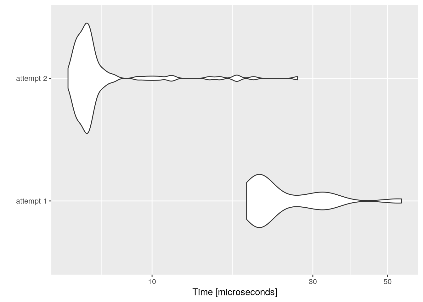

We can see graphically the superior performance of to_binary_2.

Footnotes

Indeed in many of the tracks and in computer science in general.↩︎
Since \(17 = 16 + 1 = 2^4 + 2^0\).↩︎
To see the full docs run ?bitwAnd in an R console.↩︎
With the convention that the bit 1 represents TRUE and 0 represents FALSE.↩︎
Note that the binary representation is left padded with zeros so the lengths match.↩︎
The output will be positive if and only if the \(i^{\text{th}}\) binary digit was a 1.↩︎
The defintion of limit as floor(log2(n)) is simply 1 less than the number of binary digits in \(n\).↩︎