2-D posterior toy example (RBF covariance)

Demonstration of posterior error bounds for a 2-D toy example, for various levels of sensor noise

In this notebook we will demonstrate the error bounds for the statFEM posterior for the toy example introduced in twoDim. We first import some required packages.

from dolfin import *
import numpy as np
import pandas as pd
import seaborn as sns
import matplotlib.cm as cm
import matplotlib.pyplot as plt
plt.rcParams['figure.figsize'] = (10,6)
from scipy.linalg import sqrtm
import sympy; sympy.init_printing()
from tqdm import tqdm
# code for displaying matrices nicely
def display_matrix(m):
    display(sympy.Matrix(m))
# import required functions from twoDim
from statFEM_analysis.twoDim import mean_assembler, kernMat, cov_assembler, m_post, gen_sensor, MyExpression, m_post_fem_assembler, c_post, c_post_fem_assembler

Since we again to not have access to the true distribution we will use the method outlined in the section 2-D prior toy example to approximate the convergence rate. We now set up the required code.

First we set up the mean and kernel functions for the random forcing term \(f\).

# set up mean and kernel functions
f_bar = Constant(1.0)

l_f = 0.4
σ_f = 0.1

def k_f(x):
    return (σ_f**2)*np.exp(-(x**2)/(2*(l_f**2)))

def m_f(x):
    return 1.0

We now set up a reference grid on which we will compare the covariance matrices.

N = 41
x_range = np.linspace(0,1,N)
grid = np.array([[x,y] for x in x_range for y in x_range])

ϵ = 0.001

We now set up the sensor grid and generate some sensor data.

%%time
s = 25
s_sqrt = int(np.round(np.sqrt(s)))
Y_range = np.linspace(0.01,0.99,s_sqrt)
Y = np.array([[x,y] for x in Y_range for y in Y_range])
J_fine = 120
np.random.seed(42)
v_dat = gen_sensor(ϵ,m_f,k_f,Y,J_fine,False,True)

CPU times: user 1min 28s, sys: 11.8 s, total: 1min 40s
Wall time: 22.1 s

We now set up a function to get the statFEM prior and posterior for a FE mesh size \(h\), using functions from twoDim.

def fem_prior(h,f_bar,k_f,grid):
    J = int(np.round(1/h))
    μ = mean_assembler(h,f_bar)
    Σ = cov_assembler(J,k_f,grid,False,True)
    return μ,Σ

def fem_posterior(h,f_bar,k_f,ϵ,Y,v_dat,grid):
    J = int(np.round(1/h))
    m_post_fem = m_post_fem_assembler(J,f_bar,k_f,ϵ,Y,v_dat)
    μ = MyExpression()
    μ.f = m_post_fem
    Σ = c_post_fem_assembler(J,k_f,grid,Y,ϵ,False,True)
    return μ,Σ

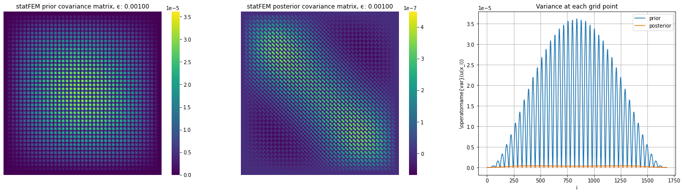
We now see if the sensor level noise causes the posterior to look different from prior.

h = 0.05
μ_prior, Σ_prior = fem_prior(h,f_bar,k_f,grid)
μ_posterior, Σ_posterior = fem_posterior(h,f_bar,k_f,ϵ,Y,v_dat,grid)

fig, (ax1,ax2,ax3) = plt.subplots(1,3,figsize=(24,6))

sns.heatmap(Σ_prior,cbar=True,
              annot=False,
              xticklabels=False,
              yticklabels=False,
              cmap=cm.viridis,
              ax=ax1)
ax1.set_title('statFEM prior covariance matrix, ϵ: %.5f' % ϵ)

sns.heatmap(Σ_posterior,cbar=True,
              annot=False,
              xticklabels=False,
              yticklabels=False,
              cmap=cm.viridis,
              ax=ax2)
ax2.set_title('statFEM posterior covariance matrix, ϵ: %.5f' % ϵ)

ax3.plot(np.diag(Σ_prior),label='prior')
ax3.plot(np.diag(Σ_posterior),label='posterior')
ax3.grid()
ax3.set_xlabel("i")
ax3.set_ylabel("\operatorname{var}(u(x_i))")
ax3.set_title("Variance at each grid point")
ax3.legend()

plt.show()

We now set up a function to compare the covariance functions on the reference grid.

def compute_cov_diff(C1,C2,tol=1e-10):
    N = np.sqrt(C1.shape[0])
    #N = C1.shape[0]
    C1_sqrt = np.real(sqrtm(C1))
    rel_error_1 = np.linalg.norm(C1_sqrt @ C1_sqrt - C1)/np.linalg.norm(C1)
    assert rel_error_1 < tol

    C12 = C1_sqrt @ C2 @ C1_sqrt
    C12_sqrt = np.real(sqrtm(C12))
    rel_error_12 = np.linalg.norm(C12_sqrt @ C12_sqrt - C12)/np.linalg.norm(C12)
    assert rel_error_12 < tol

    hSq = (1/(N-1))**2
    return hSq*(np.trace(C1) + np.trace(C2) - 2*np.trace(C12_sqrt))

We now set up a function to compute the Wasserstein distance between the statFEM posteriors.

def W(μ_1,μ_2,Σ_1,Σ_2,J_norm):
    mean_error = errornorm(μ_1,μ_2,'L2',mesh=UnitSquareMesh(J_norm,J_norm))
    cov_error = compute_cov_diff(Σ_1,Σ_2)
    cov_error = np.sqrt(np.abs(cov_error))
    error = mean_error + cov_error
    return error

In the interests of memory efficiency we will again create a function which will compute the ratios of errors by succesively refining the FE mesh as done in the section 2-D prior toy example.

def refine(h,n,f_bar,k_f,ϵ,Y,v_dat,grid,J_norm):
    # set up empty lists to hold h-values and errors (this being the ratios)
    h_range = []
    errors = []
    # get the statFEM posterior for h and h/2
    μ_1, Σ_1 = fem_posterior(h,f_bar,k_f,ϵ,Y,v_dat,grid)
    μ_2, Σ_2 = fem_posterior(h/2,f_bar,k_f,ϵ,Y,v_dat,grid)
    # compute the distance between these and store in numerator variable
    numerator = W(μ_1,μ_2,Σ_1,Σ_2,J_norm)
    # succesively refine the mesh by halving and do this n times
    for i in tqdm(range(n)):
        # store mean and cov for h/2 in storage for h
        μ_1, Σ_1 = μ_2, Σ_2
        # in storage for h/2 store mean and cov for h/4
        μ_2, Σ_2 = fem_posterior(h/4,f_bar,k_f,ϵ,Y,v_dat,grid)
        # compute the distance between the posteriors for h/2 and h/4
        # and store in denominator variable
        denominator = W(μ_1,μ_2,Σ_1,Σ_2,J_norm)
        # compute the ratio and store in error
        error = numerator/denominator
        # append the current value of h and the ratio
        h_range.append(h)
        errors.append(error)
        # store denominator in numerator and halve h
        numerator = denominator
        h = h/2
    # return the list of h-values together with the ratios for these values
    return h_range,errors

We now set up a list of starting \(h\) values and number of refinements \(n\) to get a decent number of ratios to approximate \(p\). We also set up the J_norm variable needed to control the grid on which the mean error is computed in the Wasserstein distance.

my_list = [(0.25,4),(0.2,3),(0.175,3),(0.176,3),(0.177,3),(0.178,3),(0.179,3),(0.18,3),(0.21,3),(0.215,3),(0.1,2),(0.3,4),(0.31,4),(0.315,4),(0.24,3),(0.245,3),(0.14,2),(0.16,2),(0.15,2)]
J_norm = 40

We now compute the results:

%%time
h_range = []
errors = []
np.random.seed(235)
for h,n in tqdm(my_list,desc='Outer loop'):
    h_range_tmp, errors_tmp = refine(h,n,f_bar,k_f,ϵ,Y,v_dat,grid,J_norm)
    h_range.extend(h_range_tmp)
    errors.extend(errors_tmp)

CPU times: user 16h 51min 12s, sys: 1d 13h 56min 24s, total: 2d 6h 47min 36s
Wall time: 7h 9min 40s

We now sort these results by \(h\).

h_range_array = np.array(h_range)
errors_array = np.array(errors)

argInd = np.argsort(h_range_array)
hs = h_range_array[argInd]
es = errors_array[argInd]
hs,hs_ind = np.unique(hs,return_index=True)
es = es[hs_ind]

We now plot the base-2 logarithm of the ratios against \(h\) below:

plt.plot(hs,np.log2(es),c='r')
plt.xlabel('$h$')
plt.ylabel('$\operatorname{LR}(h)$')
plt.title('Base-2 log plot of the ratios against $h$')
plt.hlines(2.0,hs[0],hs[-1],colors='black',linestyles='--')
plt.xlim(hs[-1],hs[0])
plt.grid()
plt.show()

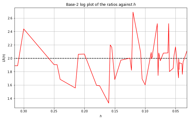
We can see from the above plot that the logarithms seems to be approaching \(p=2\) as \(h\) gets small just as predicted. However, the results aren’t that smooth and they haven’t seemed to settle on \(p=2\) yet. This can be due to memory constraints meaning we cannot use small enough \(h\). We thus smooth the above results by taking a cumulative average of the ratios and then applying \(\log_2\). We take the rolling average starting with large \(h\). We choose a cut-off point of \(h=0.15\), i.e. we discard any results for \(h>0.15\).

The results are shown below:

From the smoothed results above we can see more clearly that the ratios are converging to around \(p=2\).

# get the cumulative average of es:
i = -18
es_trimmed = es[:i]
HS = hs[:i]
pos = np.arange(0,35,step=5)
es_av = np.log2(np.cumsum(es_trimmed[::-1])/np.arange(1,len(es_trimmed)+1))
plt.plot(es_av,c='r')
plt.hlines(2.0,0,len(es_av),colors='black',linestyles='--')
plt.xticks(pos,HS[::-1][pos])
plt.xlabel('index')
plt.title('Base-2 logarithms of the cumulative averages of the ratios for $h\leq 0.15$')
plt.grid()
plt.show()

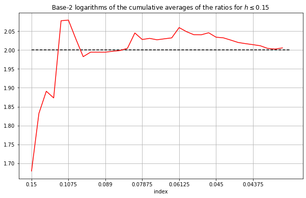
From the smoothed results above we can see more clearly that the ratios are converging to around \(p=2\). In fact, discarding the values corresponding to \(h>0.15\) seems to result in the the rolling average converging to a value slightly greater than \(2\).